Asset Allocation Bi-Weekly – Real Income versus the Wealth Effect; What is Driving Consumption? (January 24, 2022)

by the Asset Allocation Committee | PDF

One of the debates within economics is whether consumption is driven by income or wealth.  The outcome of this debate is important for policymakers; if the goal of policy is lifting or constraining growth, knowing which factor is more important to consumption is critical.  For example, if the goal is lifting economic activity and incomes are more important to consumption, transfer payments and tax cuts to lower-income households would be effective.  On the other hand, if the wealth effect[1] has a stronger impact, the same goal might be better achieved with capital gains tax cuts and interest rate reductions.

Until the mid-1990s, the evidence strongly suggested that income was much more important than the wealth effect.  But, since the mid-1990s, consumption has been much more sensitive to net worth.

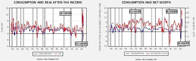
We measure consumption by the contribution to real GDP on a rolling four-quarter basis.  Disposable real income is the yearly change to overall income on an inflation-adjusted basis on an after-tax basis.  Net worth is the yearly change in assets less liabilities.  From 1947 through 2019, the correlation between consumption and real disposable income was 69.6%.  Comparing that to the impact of net worth, from 1947 through 1994, changes in net worth had only a modest positive impact on consumption; the two variables only were correlated by 12.9%.  However, from 1995 through 2019, the correlation jumped to 75.8%.

Why did net worth become more important to consumption?  We suspect there were at least two significant factors that changed the impact of the wealth effect.  The first was the expansion of defined contribution pension plans.  Households rarely saw the wealth they were accumulating under defined benefit plans.  Only at retirement would they see what they would receive from their years of saving.  Thus, rarely did they have knowledge of their accumulating wealth.  But, under defined contribution plans, households could easily see the wealth they were accumulating.  As a result of the bull markets in stocks and bonds in the 1990s, households felt “richer” and thus adjusted their spending to their expanding retirement accounts.  Second, for most households, the largest asset they hold is their homes.

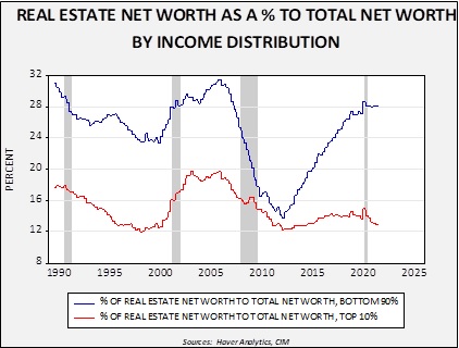
This chart shows real estate net worth compared to total net worth for the top 10% of households in the income distribution compared to the bottom 90%.  Note that 90% of households have a much higher percentage of their net worth tied to residential real estate.

Until the mid-1980s, it was difficult to access the wealth in a home until the financial services industry made refinancing a simpler process.  The ability to tap home equity is partly related to home prices.  Although amortization will gradually increase the homeowner’s share of equity, immediate changes in home prices would have a bigger impact on the net worth from real estate.  And, since in the early years of a mortgage most of a mortgage payment is applied to interest, weakening home values can have a detrimental impact on the wealth effect.  Mortgage lending is leveraged; a “prudent” loan is 80% loan to value, so small changes in home prices can have outsized effects on the net worth of the bottom 90% of households.


Returning to the first chart, we have isolated the period after the pandemic.  What is remarkable is that the relationship between real disposable income and consumption has become negative; this is likely a fluke, a function of a rapid increase in income in the form of transfer payments at a time when spending was limited due to the pandemic.  As more goods and services became available, spending has recovered.  Meanwhile, fewer transfer payments have led to falling real disposable income.  This situation will eventually normalize but still suggests that, in the short run, policies that affect real disposable income may not have much impact on consumption.  At the same time, the relationship between net worth and consumption has risen to 95.3%.  This rise may represent the fact that the aforementioned savings found a home in the asset markets.  This outcome, too, may be a decline to pre-pandemic levels, but we expect the relationship to remain strong.


Although the current relationships between real disposable income, net worth, and consumption may be temporary, for now, we can only assume they will remain dominant.  This means that policymakers face a potential risk as they move to tighten policy.  If rising interest rates weaken asset markets, the impact on consumption could be stronger than expected.  It might even lead investors to hold even more liquidity in part due to (a) fears of further declines in asset values and (b) due to the higher compensation for holding cash.  Given that 90% of households will probably be more sensitive to home prices, actions that affect home values may have an unexpectedly large impact on economic behavior.


Although our outlook for 2022 assumed no rate hikes, comments from FOMC members suggest our position is probably wrong, and policy tightening is coming.  We will be watching the path of home prices especially, but asset prices in general, to gauge the effects on consumption.  Given the FOMC’s sensitivity to asset prices, weakness in housing prices or equities could cool the ardor to tighten policy.

View PDF


[1] The wealth effect measures how much consumption is affected by changes in net worth.

Asset Allocation Bi-Weekly – The Path of Monetary Policy (January 10, 2022)

by the Asset Allocation Committee | PDF

Our expectation of no policy rate hikes this year is an out-of-consensus call in our 2022 Outlook: The Year of Fat Tails.  There are a couple of factors that suggest rate hikes this year.  First, financial markets have factored in rate hikes.  Fed funds futures suggest a greater than 50% likelihood of a rate hike beginning with the March 2022 meeting and have discounted the same likelihood for four 25 bps rate hikes by December.   Second, the Mankiw Rule, a derivation of the Taylor Rule, indicates the FOMC is hopelessly behind the curve in terms of rate hikes.

We have created five variations of the Mankiw rule, which calculates a fair value policy rate from core CPI and various measures of the labor market.  The most conservative measure puts the recommended fed funds rate at 4.33%; the most radical is 9.27%.

So, given this strong evidence, what is the argument for steady policy?    Part of the reason the Mankiw variations are so high is due to elevated inflation.  Base effects alone should lead to lower readings on inflation by mid-year, which should cool the impetus for policy tightening.  Although the labor markets show signs of being tight, the labor force remains well below pre-pandemic levels.  It may give FOMC members pause, worried that tightening could be premature.

This chart compares the three-month average of the labor force relative to its most recent peak.  The drop in the labor force seen during the pandemic was unprecedented in the post-war era.  It is uncertain whether the labor market has been permanently impaired by the pandemic.  It may never return to pre-pandemic levels.  It is also possible that as the pandemic steadily shifts to endemic, workers will return.  Thus, tightening could prematurely put this return at risk.

Another characteristic of the FOMC since Greenspan has been the attention paid to financial markets.  The concept of the “Greenspan put,” which has been attributed to every Fed chair since Greenspan, suggests a pattern where monetary policy is eased to quell turmoil in financial markets.

One clear measure of financial stress is the VIX, which measures the implied volatility of the S&P 500.  In general, the FOMC tends to avoid tightening when the 12-week average of the VIX is above 20.  For example, after the Fed raised rates in late 2015, policy remained on hold until the VIX fell decidedly.  With the VIX currently holding around 20, we expect the FOMC to delay any moves to raise rates until market volatility eases.

Finally, we suspect financial markets are underappreciating the degree of fiscal tightening that will occur this year.

Fiscal spending during the pandemic was extraordinary.  However, as that support winds down, it will act as a drag on economic growth.  If the FOMC tightens into this austerity, economic growth could weaken more than expected.  The consensus real GDP growth for 2022 is 3.9%.  That could be at risk if the Fed tightens into falling fiscal support.

Obviously, we could be wrong on our monetary policy call, and if we are, we will adjust.  For now, we think there is a case that the market is overestimating the degree of monetary policy tightening that will occur.  If we are correct, it’s likely supportive for equities, short-duration fixed income, commodities, and bearish for the dollar.

View PDF

Asset Allocation Weekly (January 8, 2021)

by Asset Allocation Committee | PDF

Although U.S. equity markets appear richly valued based on historical metrics, relative to interest rates, current values of relative earnings or sales are not extreme.  Thus, the direction of interest rates and, more specifically, the direction of monetary policy, is a key element in equity values going forward.  In other words, when does the Fed raise rates?

Over the past year, the FOMC has changed its reaction function.  Since Volcker, the Fed has tended to tighten policy before full employment is achieved to “preempt” potential inflation.  This policy has led analysts to focus on various forms of the “Taylor Rule,” which attempts to calculate the neutral rate of interest given the level of current inflation, the inflation target, and the level of slack in the economy.  That policy has ended and has been replaced with a policy that promises to keep rates low until price levels above 2% annual growth are sustained.

Of course, the actual path of policy will be determined by the “buy-in” from the members of the FOMC.  Although Chair Powell’s comments suggest he is fully committed to the new policy, it is not clear if it has universal acceptance.  At this juncture, there are no dissents, but if inflation starts to rise, we could see some of the more traditional hawks grow uncomfortable with ZIRP.  Since an uptick in inflation in 2021 is possible, given base effects alone, it does raise the question—will the Fed stay committed to low rates?

Obviously, it would be foolhardy to claim that rates will stay near zero forever, but it would make sense to have some idea of how long we can comfortably expect ZIRP to remain in place.  First, for 2021, based on the composition of the FOMC, we can reasonably expect steady policy.

The above table shows the current members of the FOMC.  The committee consists of seven governors and 12 regional Fed bank presidents.  The governors are permanent voters as is the president of the New York FRB.  Each year, four regional bank presidents also formally vote on policy.  Our table shows the current governors on top and the regional presidents below.  We rate each on our “hawk/dove” scale and have also categorized them by policy inclination.  Moderates and Traditional Hawks rely on standard economic measures to set policy; the Hawks are more inclined to raise rates preemptively, whereas the Moderates tend to have higher tolerance for inflation uncertainty.  Doves tend to only raise rates if the evidence is overwhelming for inflation.  The Financial Sensitives will entertain rate hikes or other austerity measures when financial markets appear to be overheating.  Otherwise, they tend to side with the Doves.  We have also updated our estimates, with Powell and Clarida becoming more dovish.  The addition of Governor Waller and the current roster of regional FRB presidents make it clear that the new FOMC is much more dovish than in 2020.  That would suggest policy will remain steady with a bias for additional easing.

The other factor of note we find important is the relationship of the two-year deferred Eurodollar futures relative to fed funds.  The current implied yield of the deferred Eurodollar futures suggests the market expects steady policy for the next 18 to 24 months.

Under normal circumstances, the implied deferred yield is higher than fed funds.  In periods where the implied yield falls below fed funds, shown by a vertical line, policy easing tends to occur shortly thereafter.  From 2007 into 2013, the level of the implied yield remained stubbornly elevated relative to the fed funds target, suggesting the financial markets didn’t trust the promises of Chair Bernanke to keep rates low.  It wasn’t until early 2013 that markets finally accepted that policy would stay steady (and then Bernanke blew it up by announcing the slowing of the balance sheet expansion in 2013).  Note the current level of the fed funds target and the implied LIBOR rate.  The market completely believes the Fed will keep rates low for at least the next 18 to 24 months.

Overall, with equity valuations high, the key to maintaining these lofty expectations is the level of interest rates.  As long as dovish expectations for monetary policy remain in place, these valuations will likely persist.

View PDF